Pandas
Pandas is an open-source Python Library providing high-performance data manipulation and analysis tool using its powerful data structures.
This tool is essentially your data’s home. Through pandas, you get acquainted with your data by cleaning, transforming, and analyzing it.
For example, say you want to explore a dataset stored in a CSV on your computer. Pandas will extract the data from that CSV into a DataFrame — a table, basically — then let you do things like:
- Calculate statistics and answer questions about the data, like
- What's the average, median, max, or min of each column?
- Does column A correlate with column B?
- What does the distribution of data in column C look like?
- Clean the data by doing things like removing missing values and filtering rows or columns by some criteria
- Visualize the data with help from Matplotlib. Plot bars, lines, histograms, bubbles, and more.
- Store the cleaned, transformed data back into a CSV, other file or database
Import Pandas
import pandas as pd
Core components of pandas: Series and DataFrames
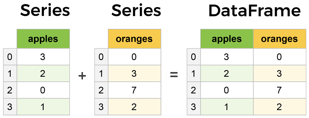
The primary two components of pandas are the Series and DataFrame.
A Series is essentially a column, and a DataFrame is a multi-dimensional table made up of a collection of Series.
DataFrames and Series are quite similar in that many operations that you can do with one you can do with the other, such as filling in null values and calculating the mean.
Series
Series is a one-dimensional labeled array capable of holding data of any type (integer, string, float, python objects, etc.). The axis labels are collectively called index.
pandas.Series( data, index, dtype, copy)
data - data takes various forms like ndarray, list, constants index - Index values must be unique and hashable, same length as data. Default np.arrange(n) if no index is passed. dtype - dtype is for data type. If None, data type will be inferred copy - Copy data. Default False
colors = pd.Series(["Red", "Green", "Blue"])
colors
0      Red
1    Green
2     Blue
dtype: object
cars = pd.Series(["Audi", "Ferrai", "BMW"])
cars
0      Audi
1    Ferrai
2       BMW
dtype: object
import numpy as np
data = np.array(['a','b','c','d'])
s = pd.Series(data,index=[100,101,102,103])
100  a
101  b
102  c
103  d
dtype: object
data = {'a' : 0., 'b' : 1., 'c' : 2.}
s = pd.Series(data)
a 0.0
b 1.0
c 2.0
dtype: float64
s = pd.Series(5, index=[0, 1, 2, 3])
print s
0  5
1  5
2  5
3  5
dtype: int64
#retrieve the first element
s[0]

#retrieve the first three element
s[:3]

#retrieve the last three element
s[-3:]

#Retrieve a single element using index label value.
s['a']

#Retrieve multiple elements using a list of index label values.
s[['a','c','d']]
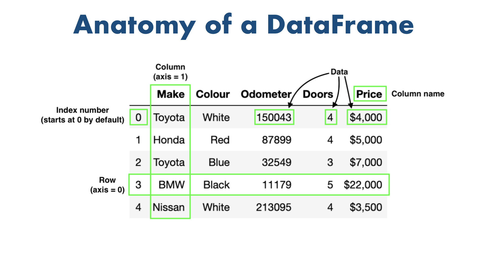
DataFrames
A Data frame is a two-dimensional data structure, i.e., data is aligned in a tabular fashion in rows and columns.
pandas.DataFrame( data, index, columns, dtype, copy)
data - data takes various forms like ndarray, series, map, lists, dict, constants and also another DataFrame. index- For the row labels, the Index to be used for the resulting frame is Optional Default np.arange(n) if no index is passed. columns - For column labels, the optional default syntax is - np.arange(n). This is only true if no index is passed. dtype - Data type of each column. copy - This command (or whatever it is) is used for copying of data, if the default is False.
A pandas DataFrame can be created using various inputs like −
- Lists
- dict
- Series
- Numpy ndarrays
- Another DataFrame
dataframes = pd.DataFrame({ "color": colors, "car": cars })
dataframes
| color | car | |
|---|---|---|
| 0 | Red | Audi |
| 1 | Green | Ferrai |
| 2 | Blue | BMW |
data = {'Name':['Tom', 'Jack', 'Steve', 'Ricky'],'Age':[28,34,29,42]}
df = pd.DataFrame(data, index=['rank1','rank2','rank3','rank4'])
df
         Age    Name
rank1    28      Tom
rank2    34     Jack
rank3    29    Steve
rank4    42    Ricky
data = [{'a': 1, 'b': 2},{'a': 5, 'b': 10, 'c': 20}]
df = pd.DataFrame(data)
print df
    a    b      c
0   1   2     NaN
1   5   10   20.0
Column Operations
# select column
df['one']

# delete column
del df['one']
df.pop('two')

# add column
df['three']=pd.Series([10,20,30],index=['a','b','c'])
df['four']=df['one']+df['three']
Row Operations
# select row
df.loc['b'] # Selection by Label
df.iloc[2]  # Selection by integer location

# Slice Rows
df[2:4]

# Addition of Rows
df = df.append(df2)

# Drop rows with label 0
df.drop(0)
CSVs
Load CSV data
# import data
car_sales = pd.read_csv("car-sales.csv")
car_sales
| Make | Colour | Odometer (KM) | Doors | Price | |
|---|---|---|---|---|---|
| 0 | Toyota | White | 150043 | 4 | $4,000.00 |
| 1 | Honda | Red | 87899 | 4 | $5,000.00 |
| 2 | Toyota | Blue | 32549 | 3 | $7,000.00 |
| 3 | BMW | Black | 11179 | 5 | $22,000.00 |
| 4 | Nissan | White | 213095 | 4 | $3,500.00 |
| 5 | Toyota | Green | 99213 | 4 | $4,500.00 |
| 6 | Honda | Blue | 45698 | 4 | $7,500.00 |
| 7 | Honda | Blue | 54738 | 4 | $7,000.00 |
| 8 | Toyota | White | 60000 | 4 | $6,250.00 |
| 9 | Nissan | White | 31600 | 4 | $9,700.00 |
Describe Data
# Attributes
car_sales.dtypes
Make             object
Colour           object
Odometer (KM)     int64
Doors             int64
Price            object
dtype: object
car_sales.columns
# Index(['Make', 'Colour', 'Odometer (KM)', 'Doors', 'Price'], dtype='object')

car_sales.index
# RangeIndex(start=0, stop=10, step=1)

car_sales["Doors"].mean()
# 4.0

car_sales["Doors"].sum()
# 40

len(car_sales)
# 10

car_sales.info()
#  #   Column         Non-Null Count  Dtype
# ---  ------         --------------  -----
# dtypes: int64(2), object(3)
# memory usage: 528.0+ bytes
# Functions
car_sales.describe() # give min max mean and other info of numerical data
Selecting and Viewing data
car_sales.head(5) # gives small snapshot of top 5 lines of the data
car_sales.tail(5) # gives small snapshot of bottom 5 lines of the data
animals = pd.Series(["cat", "dog", "bird", "panda", "snake"], [0, 3, 9, 8, 5])
# 0      cat
# 3      dog
# 9     bird
# 8    panda
# 5    snake

animals.loc[3] # loc refers to the value of index
# 'dog'
animals.iloc[3] # iloc refers to the position of index
# panda
car_sales[car_sales["Make"] == "Toyota"]
car_sales[car_sales["Odometer (KM)"] > 100000]